
Because analyses of variance (ANOVA) isn’t a built-in tool, Excel doesn’t produce the descriptive statistics for each combination of conditions. You have to have those statistics (means and standard errors) to create a chart of the results.
This, of course, isn’t hard to do. The following shows the table of means and the table of standard errors along with the data. Each entry in the means table is just the AVERAGE function applied to the appropriate cell range. So the value in D13 is
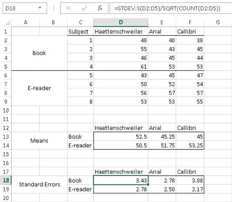
=AVERAGE(D2:D5)
Each entry in the Standard Errors table is the result of applying three functions to the appropriate cell range. For example, select D18 so that its value appears in the Formula bar in the figure:
=STDEV.S(D2:D5)/SQRT(COUNT(D2:D5))
The following figure shows the column chart for the results. To create it, select the means table (C12:F14) and select Insert | Recommended Charts and then select the Clustered Column option. Then add the error bars for the standard errors and tweak the chart.
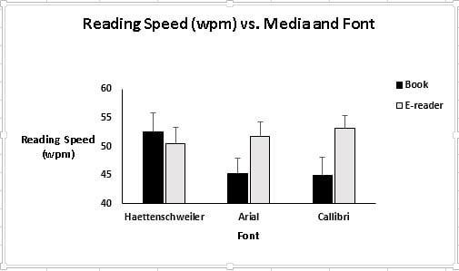
The chart clearly illustrates the Media X Font interaction. For Haettenschweiler, the reading speed is higher for the book. For each of the others, the reading speed is higher with the e-reader.