
Although it may seem daunting, graphing polynomials is a pretty straightforward process. Once you have found the zeros for a polynomial, you can follow a few simple steps to graph it.
For example, if you have found the zeros for the polynomial f(x) = 2x4 – 9x3 – 21x2 + 88x + 48, you can apply your results to graph the polynomial, as follows:
Plot the x- and y-intercepts on the coordinate plane.
Use the rational root theorem to find the roots, or zeros, of the equation, and mark these zeros. In this example, they are x = –3, x = –1/2, and x = 4. These are the x-intercepts.
Now plot the y-intercept of the polynomial. The y-intercept is always the constant term of the polynomial — in this case, y = 48. If no constant term is written, the y-intercept is 0.
Determine which way the ends of the graph point.
You can use a handy test called the leading coefficient test, which helps you figure out how the polynomial begins and ends. The degree and leading coefficient of a polynomial always explain the end behavior of its graph:
If the degree of the polynomial is even and the leading coefficient is positive, both ends of the graph point up.
If the degree is even and the leading coefficient is negative, both ends of the graph point down.
If the degree is odd and the leading coefficient is positive, the left side of the graph points down and the right side points up.
If the degree is odd and the leading coefficient is negative, the left side of the graph points up and the right side points down.
The figure displays this concept in correct mathematical terms.
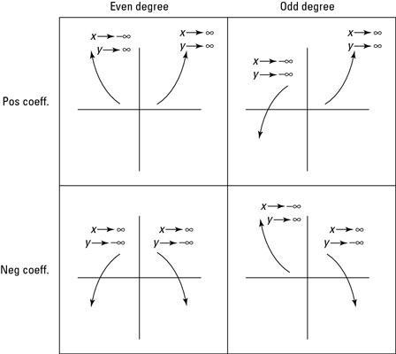
The function f(x) = 2x4 – 9x3 – 21x2 + 88x + 48 is even in degree and has a positive leading coefficient, so both ends of its graph point up (they go to positive infinity).
Figure out if the graph lies above or below the x-axis between each pair of consecutive x-intercepts by picking any value between these intercepts and plugging it into the function.
You can either simplify each one or just figure out whether the end result is positive or negative. For now, you don’t really care about the exact look of the graph. (In calculus, you learn how to find additional values that lead to a more accurate graph.)
A graphing calculator gives a very accurate picture of the graph. Calculus allows you to find the relative max and min exactly, using an algebraic process, but you can often use the calculator to find them. You can use your graphing calculator to check your work and make sure the graph you’ve created looks like the one the calculator gives you.
Using the zeros for the function, set up a table to help you figure out whether the graph is above or below the x-axis between the zeros. Here is the table for this example:
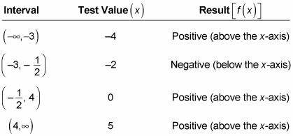
The first interval,
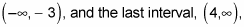
both confirm the leading coefficient test from Step 2 — this graph points up (to positive infinity) in both directions.
Plot the graph.
Now that you know where the graph touches the x-axis, how the graph begins and ends, and whether the graph is positive (above the x-axis) or negative (below the x-axis), you can sketch out the graph of the function. Typically, in pre-calculus, this information is all you want or need when graphing. Calculus does show you how to get several other useful points that create an even better graph. If you want, you can always pick more points in the intervals and graph them to get a better idea of what the graph looks like. This figure shows the completed graph.
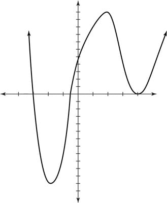 Graphing the polynomial f(x) = 2x4 – 9x3 – 21x2 + 88x + 48.
Did you notice that the double root (with multiplicity two) causes the graph to “bounce” on the x-axis instead of actually crossing it? This is true for any root with even multiplicity. For any polynomial, if the root has an odd multiplicity at root c, the graph of the function crosses the x-axis at x = c. If the root has an even multiplicity at root c, the graph meets but doesn’t cross the x-axis at x = c.