


Panes are great for viewing different parts of the same worksheet that normally can’t be seen together in Excel 2013. You can also use panes to freeze headings in the top rows and first columns so that the headings stay in view at all times, no matter how you scroll through the worksheet.
Frozen headings are especially helpful when you work with a table that contains information that extends beyond the rows and columns shown onscreen.
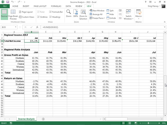
The Income Analysis worksheet contains more rows and columns than you can see at one time (unless you decrease the magnification to about 40% with Zoom, which makes the data too small to read). In fact, this worksheet continues down to row 52 and over to column P.
By dividing the worksheet into four panes between rows 2 and 3 and columns A and B and then freezing them on the screen, you can keep the column headings in row 2 that identify each column of information on the screen while you scroll the worksheet up and down to review information on income and expenses.
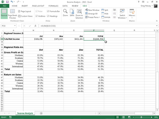
Additionally, you can keep the row headings in column A on the screen while you scroll the worksheet to the right.
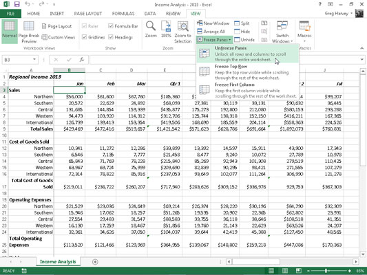
To create and freeze these panes, follow these steps:
Position the cell cursor in cell B3.
Click View→Freeze Panes on the Ribbon and then click Freeze Panes on the drop-down menu or press Alt+WFF.
In this example, Excel freezes the top and left pane above row 3 and left of column B.
When Excel sets up the frozen panes, the borders of frozen panes are represented by a single line rather than the thin gray bar, as is the case when simply splitting the worksheet into panes.
See what happens when you scroll the worksheet up after freezing the panes. Below, you can see the worksheet so that rows 33 through 52 of the table appear under rows 1 and 2. Because the vertical pane with the worksheet title and column headings is frozen, it remains onscreen. (Normally, rows 1 and 2 would have been the first to disappear when you scroll the worksheet up.)
See what happens when you scroll the worksheet to the right. Here, the worksheet is scrolled so that the data in columns M through P appear after the data in column A. Because the first column is frozen, it remains onscreen, helping you identify the various categories of income and expenses for each month.
Click Freeze Top Row or Freeze First Column on the Freeze Panes button’s drop-down menu to freeze the column headings in the top row of the worksheet or the row headings in the first column of the worksheet, regardless of where the cell cursor is located in the worksheet.
To unfreeze the panes in a worksheet, click View→Freeze Panes on the Ribbon and then click Unfreeze Panes on the Freeze Panes button’s drop-down menu or press Alt+WFF. Choosing this option removes the panes, indicating that Excel has unfrozen them.
Did this glimpse into Excel data management leave you longing for more information and insight about Microsoft's popular spreadsheet program? You're free to test drive any of the For Dummies eLearning courses. Pick your course (you may be interested in more from Excel 2013), fill out a quick registration, and then give eLearning a spin with the Try It! button. You'll be right on course for more trusted know how: The full version's also available at Excel 2013.

