You can and will want to format the information contained in an Excel pivot table. Essentially, you have two ways of doing this: using standard cell formatting and using an autoformat for the table.
Using standard cell formatting
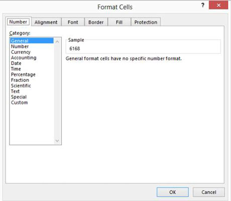
To format a single cell or a range of cells in your pivot table, select the range, right-click the selection, and then choose Format Cells from the shortcut menu. When Excel displays the Format Cells dialog box, use its tabs to assign formatting to the selected range.
For example, if you want to assign numeric formatting, click the Number tab, choose a formatting category, and then provide any other additional formatting specifications appropriate — such as the number of decimal places to be used.
Using PivotTable styles for automatic formatting
You can also format an entire pivot table. Just select the Design tab and then click the command button that represents the predesigned PivotTable report format you want. Excel uses this format to reformat your pivot table information.
If you don’t look closely at the Design tab, you might not see something that’s sort of germane to this discussion of formatting PivotTables: Excel provides several rows of PivotTable styles. Do you see the scrollbar along the right edge of this part of the ribbon?
If you scroll down, Excel displays a bunch more rows of predesigned PivotTable report formats — including some report formats that just go ape with color. And if you click the More button below the scroll buttons, the list expands so you can see the Light, Medium, and Dark categories.
Using the Other Design tab tools
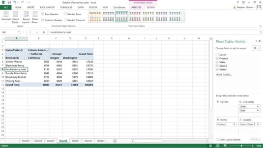
The Design tab provides several other useful tools you can use with your pivot tables. For example, the tab’s ribbon includes Subtotals, Grand Totals, Report Layout, and Blank Rows command buttons. Click one of these buttons and Excel displays a menu of formatting choices related to the command button’s name.
If you click the Grand Totals button, for example, Excel displays a menu that lets you add and remove grand total rows and columns to the PivotTable.
Finally, just so you don’t miss them, notice that the PivotTable Tools Design tab also provides four check boxes — Row Headers, Column Headers, Banded Rows, and Banded Columns — that also let you change the appearance of your PivotTable report. If the check box labels don’t tell you what the box does, just experiment. You’ll easily figure things out, and you can’t hurt anything by trying.