
If you’re working with a large table of data in Excel 2010, you can apply number filters to columns that contain values to temporarily hide unwanted values. Excel provides several options for filtering numeric data, including filtering for top or bottom values (using the Top 10 option) or filtering for values that are above or below the average in a column that contains numeric data.
Excel 2010 tables automatically display filter arrows beside each of the column headings. To display the filter arrows so that you can filter data, format a range as a table using the Table button on the Insert tab. Or, you can click the Filter button in the Sort & Filter group on the Data tab.
Filtering for top or bottom values
Follow these steps to filter for the top or bottom numbers in a table:
Click the filter arrow for the numeric column by which you want to filter data.
The filter drop-down list appears.
Point to Number Filters in the drop-down list.
Choose Top 10 in the resulting menu.
The Top 10 AutoFilter dialog box appears.
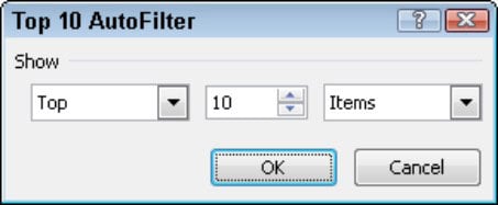 Use the Top 10 AutoFilter dialog box to filter on top or bottom values in a table.
From the first option, select whether you want the Top (highest) or Bottom (lowest) values.
In the second option, select the number of items you want to see (from 1 to 500).
This spin box displays a default value of 10.
In the third option, select whether you want to filter the items by their names or by their percentiles.
For example, choose to list the top 10 customers per their sales dollars, or list the top 10% of your customer base.
Click OK.
Excel displays the records that match your criteria.
Filtering for above- or below-average values
Use these steps to filter a table for above-average or below-average values in a column:
Click the filter arrow for the numeric column by which you want to filter data.
The filter drop-down list appears.
Point to Number Filters in the drop-down list.
Choose Above Average or Below Average in the resulting menu to filter by numbers that meet either condition.
Only the records with values above or below the total average (for that column) appear in the filtered list.
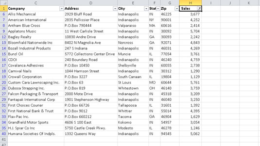 A Below Average filter applied to a column of numeric data in a table.
To remove filters and redisplay all table data, click the Clear button on the Data tab. If multiple columns are filtered, you can click a filter arrow and select Clear Filter to remove a filter from that column only. To remove the filter arrows when you’re done filtering data, choose Filter in the Sort & Filter group of the Data tab (or press Ctrl+Shift+L).