How to Derive the Schrödinger Equation

In quantum physics, the Schrödinger technique, which involves wave mechanics, uses wave functions, mostly in the position basis, to reduce questions in quantum physics to a differential equation.

Werner Heisenberg developed the matrix-oriented view of quantum physics, sometimes called matrix mechanics. The matrix representation is fine for many problems, but sometimes you have to go past it, as you’re about to see.

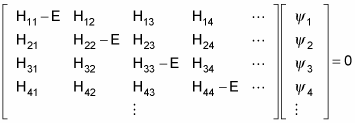
One of the central problems of quantum mechanics is to calculate the energy levels of a system. The energy operator is called the Hamiltonian, H, and finding the energy levels of a system breaks down to finding the eigenvalues of the problem:

Here, E is an eigenvalue of the H operator.

Here’s the same equation in matrix terms:

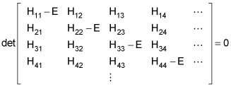
The allowable energy levels of the physical system are the eigenvalues E, which satisfy this equation. These can be found by solving the characteristic polynomial, which derives from setting the determinant of the above matrix to zero, like so

That’s fine if you have a discrete basis of eigenvectors — if the number of energy states is finite. But what if the number of energy states is infinite? In that case, you can no longer use a discrete basis for your operators and bras and kets — you use a continuous basis.

Representing quantum mechanics in a continuous basis is an invention of the physicist Erwin Schrödinger. In the continuous basis, summations become integrals. For example, take the following relation, where I is the identity matrix:

It becomes the following:

And every ket

can be expanded in a basis of other kets,

like this:

Take a look at the position operator, R, in a continuous basis. Applying this operator gives you r, the position vector:

In this equation, applying the position operator to a state vector returns the locations, r, that a particle may be found at. You can expand any ket in the position basis like this:

And this becomes

Here’s a very important thing to understand:

is the wave function for the state vector

— it’s the ket’s representation in the position basis.

Or in common terms, it’s just a function where the quantity

represents the probability that the particle will be found in the region d³r centered at r.

The wave function is the foundation of what’s called wave mechanics, as opposed to matrix mechanics. What’s important to realize is that when you talk about representing physical systems in wave mechanics, you don’t use the basis-less bras and kets of matrix mechanics; rather, you usually use the wave function — that is, bras and kets in the position basis.

Therefore, you go from talking about

This wave function is just a ket in the position basis. So in wave mechanics,

becomes the following:

You can write this as the following:

But what is

It’s equal to

The Hamiltonian operator, H, is the total energy of the system, kinetic (p²/2m) plus potential (V(r)) so you get the following equation:

But the momentum operator is

Therefore, substituting the momentum operator for p gives you this:

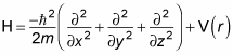
Using the Laplacian operator, you get this equation:

You can rewrite this equation as the following (called the Schrödinger equation):

So in the wave mechanics view of quantum physics, you’re now working with a differential equation instead of multiple matrices of elements. This all came from working in the position basis,

When you solve the Schrödinger equation for

you can find the allowed energy states for a physical system, as well as the probability that the system will be in a certain position state.

Note that, besides wave functions in the position basis, you can also give a wave function in the momentum basis,

or in any number of other bases.