
When creating a one-variable data table in Excel 2013, you designate one cell in the worksheet that serves either as the Row Input Cell (if you’ve entered the series of possible values across columns of a single row) or as the Column Input Cell (if you’ve entered the series of possible values down the rows of a single column).
Below you see a 2014 sales projections spreadsheet for which a one-variable data table is to be created. In this worksheet, the projected sales amount in cell B5 is calculated by adding last year’s sales total in cell B2 to the amount that it is expected to grow in 2014 (calculated by multiplying last year’s total in cell B2 by the growth percentage in cell B3), giving you the formula
=B2+(B2*B3)
Because the Create From Selection command button is clicked on the Ribbon’s Formulas tab after making A2:B5 the selection and accepted the Left Column check box default, the formula uses the row headings in column A and reads:
=Sales_2013+(Sales_2013*Growth_2014)
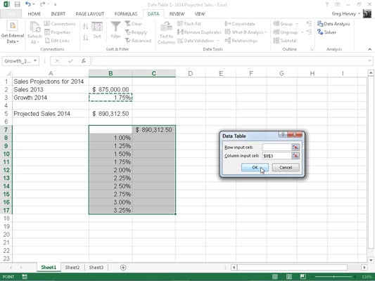
As you can see below, a column was entered of possible growth rates ranging from 1% all the way to 5.5% down column B in the range B8:B17. To create the one-variable data table that plugs each of these values into the sales growth formula, follow these simple steps:
Copy the original formula entered in cell B5 into cell C7 by typing = (equal to) and then clicking cell B5 to create the formula =Projected_Sales_2014.
The copy of the original formula (to substitute the series of different growth rates in B8:B17 into) is now the column heading for the one-variable data table.
Select the cell range B7:C17.
The range of the data table includes the formula along with the various growth rates.
Click Data→What-If Analysis→Data Table on the Ribbon.
Excel opens the Data Table dialog box.
Click the Column Input Cell text box in the Data Table dialog box and then click cell B3, the Growth_2014 cell with the original percentage, in the worksheet.
Excel inserts the absolute cell address, $B$3, into the Column Input Cell text box.
Click OK to close the Data Table dialog box.
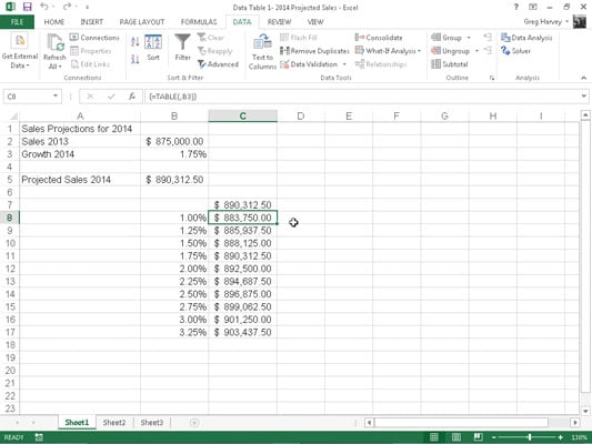
As soon as you click OK, Excel creates the data table in the range C8:C17 by entering a formula using its TABLE function into this range. Each copy of this formula in the data table uses the growth rate percentage in the same row in column B to determine the possible outcome.
Click cell C7, then click the Format Painter command button in the Clipboard group on the Home tab and drag through the cell range C8:C17.
Excel copies the Accounting number format to the range of possible outcomes calculated by this data table.
A couple of important things to note about the one-variable data table created in this spreadsheet:
If you modify any growth-rate percentages in the cell range B8:B17, Excel immediately updates the associated projected sales result in the data table. To prevent Excel from updating the data table until you click the Calculate Now (F9) or Calculate Sheet command button (Shift+F9) on the Formulas tab, click the Calculation Options button on the Formulas tab and then click the Automatic Except for Data Tables option (Alt+MXE).
If you try to delete any single TABLE formula in the cell range C8:C17, Excel displays a Cannot Change Part of a Data Table alert. You must select the entire range of formulas (C8:C17 in this case) before you press Delete or click the Clear or Delete button on the Home tab.