
Excel 2007 makes formatting a new pivot table you’ve added to a worksheet as quick and easy as formatting any other table of data. The PivotTable Tools Design tab includes special formatting options for pivot tables.
Refine the Pivot Table style
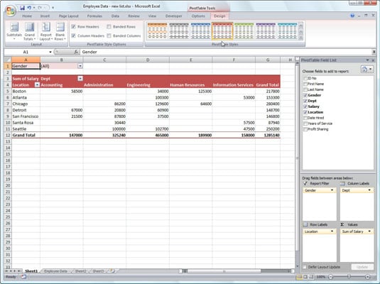
Follow these steps to apply a style to a pivot table:
Select any cell in the pivot table and click the Design tab.
The PivotTable Tools Design tab is divided into three groups:
The Layout group lets you add subtotals and grand totals to the pivot table and modify its basic layout.
The PivotTable Style Options group lets you refine the pivot table style you select for the table using the PivotTable Styles gallery to the immediate right.
The PivotTable Styles group contains the gallery of styles you can apply to the active pivot table by clicking the desired style thumbnail.
Click the More button in the PivotTable Styles group to display the PivotTable Styles gallery, and select a style.
The pivot table displays the selected style.
Refine the style using the check box options in the PivotTable Style Options group.
For example, you can add banding to the columns or rows of a style that doesn’t already use alternate shading to add more contrast to the table data by selecting the Banded Rows or Banded Columns check box.
 A pivot table formatted with Pivot Style Medium 10 in the PivotTable Styles gallery.
Keep in mind that after applying any style from the Light, Medium, or Dark group in the PivotTable Styles gallery, you can then use Live Preview to see how the pivot table would look in any style that you mouse over in the gallery.
Formatting the values in the pivot table
To format the summed values entered as the data items of the pivot table with an Excel number format, follow these steps:
Click the name of the field in the pivot table that contains the words “Sum of” and then click the Field Settings command button on the PivotTable Tools Options tab.
Excel opens the Value Field Settings dialog box.
Click the Number Format button in the Value Field Settings dialog box.
The Format Cells dialog box appears, with the Number tab displayed.
In the Category list, select the number format you want to assign.
(Optional) Modify any other options for the selected number format, such as Decimal Places, Symbol, and Negative Numbers.
Click OK two times to close both dialog boxes.