Format Tables from the Ribbon in Excel 2013

By Greg Harvey from Excel 2013 All-in-One For Dummies

Excel 2013’s Format as Table feature enables you to both define an entire range of data as a table and format all its data all in one operation. After you define a cell range as a table, you can completely modify its formatting simply by clicking a new style thumbnail in the Table Styles gallery.

Excel also automatically extends this table definition — and consequently its table formatting — to all the new rows you insert within the table and add at the bottom as well as any new columns you insert within the table or add to either the table’s left or right end.

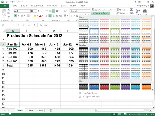
The Format as Table feature is so automatic that, to use it, you only need to position the cell pointer somewhere within the table of data prior to clicking the Format as Table command button on the Ribbon’s Home tab.

Clicking the Format as Table command button opens its rather extensive Table Styles gallery with the formatting thumbnails divided into three sections — Light, Medium, and Dark — each of which describes the intensity of the colors used by its various formats.

As soon as you click one of the table formatting thumbnails in this Table Styles gallery, Excel makes its best guess as to the cell range of the data table to apply it to (indicated by the marquee around its perimeter), and the Format As Table dialog box similar to the one shown appears.

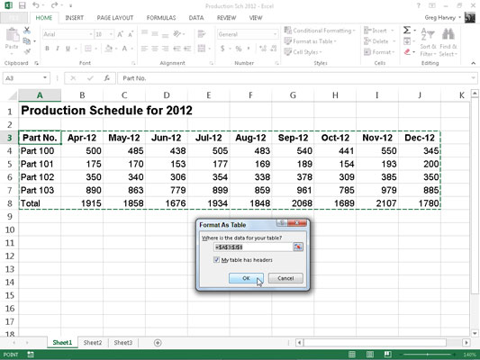
This dialog box contains a Where Is the Data for Your Table? text box that shows the address of the cell range currently selected by the marquee and a My Table Has Headers check box (selected by default).

If Excel does not correctly guess the range of the data table you want to format, drag through the cell range to adjust the marquee and the range address in the Where Is the Data for Your Table? text box.

If your data table doesn’t use column headers, click the My Table Has Headers check box to deselect it before you click the OK button — Excel will then add its own column headings (Column1, Column2, Column3, and so forth) as the top row of the new table.

Keep in mind that the table formats in the Table Styles gallery are not available if you select multiple nonadjacent cells before you click the Format as Table command button on the Home tab. You can convert only one range of cell data into a table at a time.

After you click the OK button in the Format As Table dialog box, Excel applies the format of the thumbnail you clicked in the gallery to the data table, and the command buttons on the Design tab of the Table Tools contextual tab appear on the Ribbon.

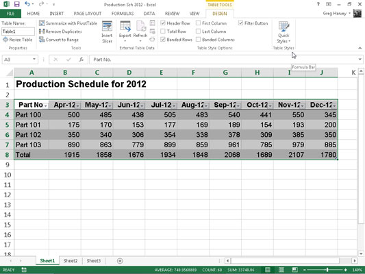
As you can see, when Excel defines a range as a table, it automatically adds AutoFilter drop-down buttons to each of the column headings (the little buttons with triangle pointing downward in the lower-right corner of the cells with the column labels).

To hide these AutoFilter buttons, click the Filter button on the Data tab or press Alt+AT. (You can always redisplay them by clicking the Filter button on the Data tab or by pressing Alt+AT a second time.)

The Design contextual tab enables you to use the Live Preview feature to see how your table data would appear in other table styles.

Simply select the Quick Styles button and then highlight any of the format thumbnails in the Table Style group with the mouse or Touch pointer to see the data in your table appear in that table format, using the vertical scroll bar to scroll the styles in the Dark section into view in the gallery.

In addition to enabling you to select a new format from the Table gallery in the Table Styles group, the Design tab contains a Table Style Options group you can use to further customize the look of the selected format. The Table Style Options group contains the following check boxes:

Header Row: Add Filter buttons to each of the column headings in the first row of the table.
Total Row: Add a Total row to the bottom of the table that displays the sum of the last column of the table (assuming that it contains values).

To apply a Statistical function other than Sum to the values in a particular column of the new Total row, click the cell in that column’s Total row. Doing this displays a drop-down list — None, Average, Count, Count Numbers, Max, Min, Sum, StdDev (Standard Deviation), or Var (Variation) — on which you click the new function to use.
Banded Rows: Apply shading to every other row in the table.
First Column: Display the row headings in the first row of the table in bold.
Last Column: Display the row headings in the last row of the table in bold.
Banded Columns: Apply shading to every other column in the table.

Keep in mind that whenever you assign a format in the Table Styles gallery to one of the data tables in your workbook, Excel automatically assigns that table a generic range name (Table1, Table2, and so on). You can use the Table Name text box in the Properties group on the Design tab to rename the data table by giving it a more descriptive range name.

When you finish selecting and/or customizing the formatting of your data table, click a cell outside of the table to remove the Design contextual tab from the Ribbon. If you later decide that you want to further experiment with the table’s formatting, click any of the table’s cells to redisplay the Design contextual tab at the end of the Ribbon.