By default, the FIND function returns the position number of the first instance of the character you are searching for. If you want the position number of the second instance, you can use the optional Start_Num argument. This argument lets you specify the character position in the text string to start the search.
For example, the following formula returns the position number of the second hyphen because you tell the FIND function to start searching at position 5 (after the first hyphen).
=FIND("-","PWR-16-Small", 5)
To use this formula dynamically (that is, without knowing where to start the search) you can nest a FIND function as the Start_Num argument in another FIND function. You can enter this formula into Excel to get the position number of the second hyphen.
=FIND("-","PWR-16-Small", FIND("-","PWR-16-Small")+1)
The figure demonstrates a real-world example of this concept.
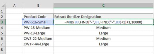
Here, you extract the size attribute from the product code by finding the second instance of the hyphen and using that position number as the starting point in the MID function. The formula shown in cell C3 is as follows:
=MID(B3,FIND("-",B3,FIND("-",B3)+1)+1,10000)
This formula tells Excel to find the position number of the second hyphen, move over one character, and then extract the next 10,000 characters. Of course, there aren’t 10,000 characters, but using a large number like that ensures that everything after the second hyphen is pulled.