
When testing a hypothesis for a small sample where you have to find the appropriate critical left-tail value, this value depends on certain criteria. In addition to being negative, the value also depends on the sample size and whether or not the population standard deviation is known.
A left-tailed test is a test to determine if the actual value of the population mean is less than the hypothesized value. (“Left tail” refers to the smallest values in a probability distribution.)
After you calculate a test statistic, you compare it to one or two critical values, depending on the alternative hypothesis, to determine whether you should reject the null hypothesis.
A critical value shows the number of standard deviations away from the mean of a distribution where a specified percentage of the distribution is above the critical value and the remainder of the distribution is below the critical value. A left-tailed test has one negative critical value, as shown here.
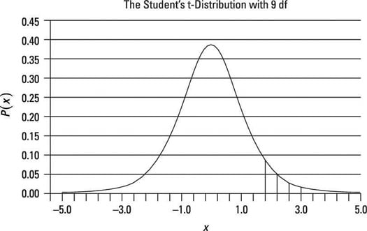
Note that a small sample is less than 30. When you use a small sample to test a hypothesis about the population mean, you take the resulting critical value from the Student’s t-distribution. In a left-tailed test, the critical value is
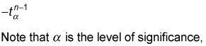
and n represents the sample size.
As an example of a left-tailed test, suppose the level of significance is 0.05 and the sample size is 10; then you get a single negative critical value:
You get this number from the t-table at the intersection of the row representing 9 degrees of freedom and the t0.05 column.
| Degrees of Freedom | t0.10 | t0.05 | t0.025 | t0.01 | t0.005 |
|---|---|---|---|---|---|
| 6 | 1.440 | 1.943 | 2.447 | 3.143 | 3.707 |
| 7 | 1.415 | 1.895 | 2.365 | 2.998 | 3.499 |
| 8 | 1.397 | 1.860 | 2.306 | 2.896 | 3.355 |
| 9 | 1.383 | 1.833 | 2.262 | 2.821 | 3.250 |
| 10 | 1.372 | 1.812 | 2.228 | 2.764 | 3.169 |
| 11 | 1.363 | 1.796 | 2.201 | 2.718 | 3.106 |
| 12 | 1.356 | 1.782 | 2.179 | 2.681 | 3.055 |
| 13 | 1.350 | 1.771 | 2.160 | 2.650 | 3.012 |
| 14 | 1.345 | 1.761 | 2.145 | 2.624 | 2.977 |
| 15 | 1.341 | 1.753 | 2.131 | 2.602 | 2.947 |
You find that the critical value is –1.833,
as shown in the figure. The shaded region in the left tail represents the rejection region; if the test statistic falls in this area, the null hypothesis will be rejected.