You can test hypotheses about two population means where the populations are independent of each other, but have equal size and variance. With equal population variances, the test statistic requires the calculation of a pooled variance — this is the variance that the two populations have in common. You use the Student's t-distribution to find the test statistic and critical values.
The choice of distribution for the hypothesis test based on independent samples is summarized in this table:
| Condition | Distribution |
|---|---|
| Equal variances | Student's t |
| Unequal variances: at least one small sample | Student's t |
| Unequal variances: large samples | Standard Normal (Z) |
If the variances of two populations are equal (or are assumed to be equal) the appropriate test statistic is based on the Student's t-distribution:
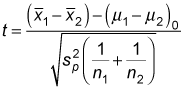
Here's what each term means:
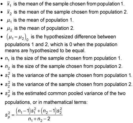
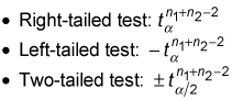
If you are conducting a hypothesis test of two population means with equal population variances, you take the critical values from the Student's t-distribution with n1 + n2 – 2 degrees of freedom, which gives you the following critical values:
As an example, say a marketing company is interested in determining whether men and women are equally likely to buy a new product. The company randomly chooses samples of men and women and asks them to assign a numerical value to their likelihood of buying the product (1 being the least likely, and 10 being the most likely).
Based on past experience, the population variances are assumed to be equal. The first step is to assign one group to be the first population ("population 1") and the other group to be the second population ("population 2"). The company designates men as population 1 and women as population 2.
The next step is to choose samples from both populations. (The sizes of these samples do not have to be equal.) Suppose that the company chooses samples of 21 men and 21 women. These samples are used to compute the sample mean and sample standard deviation for both men and women.
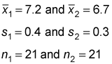
Assume that the sample mean score of the men is 7.2; the sample mean score of the women is 6.7. Also assume that the sample standard deviation of the men is 0.4, and the sample standard deviation of the women is 0.3. With this data in place, the null hypothesis that the population mean scores are equal is tested by the marketing company at the 5 percent level of significance.
You can summarize the sample data like so:
The null hypothesis is
The alternative hypothesis is
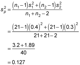
To compute the test statistic, you first calculate the pooled variance:
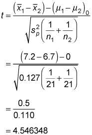
You then substitute this result into the test statistic formula:
You can find the appropriate critical values from this table (which is an excerpt from the Student's t-table).
| Degrees of Freedom | t0.10 | t0.05 | t0.025 | t0.01 | t0.005 |
|---|---|---|---|---|---|
| 30 | 1.310 | 1.697 | 2.042 | 2.457 | 2.750 |
| 40 | 1.303 | 1.684 | 2.021 | 2.423 | 2.704 |
| 60 | 1.296 | 1.671 | 2.000 | 2.390 | 2.660 |
These are found as follows. The top row of the Student's t-table lists different values of
where the right tail of the Student's t-distribution has a probability (area) equal to
In this case, alpha is 0.05; using a tail area of 0.025
and 40 degrees of freedom, you find that the critical values are:
Because the test statistic (4.546348) exceeds the positive critical value (2.021), the null hypothesis
is rejected.
With a two-tailed test, there are actually two alternatives available to the null hypothesis:
(that is, the mean rating among men is greater than the mean rating among women) or
(that is, the mean rating among men is less than the mean rating among women). In this case, the test statistic is large and positive, which suggests that the mean for men is greater than the mean for women. A large and positive test statistic indicates that the sample mean for men is significantly greater than the sample mean for women. In other words, men are more likely to buy the new product than women.