
Before getting into the closed-loop system function of the CD/DVD case study, consider a few attributes of the open-loop system function by writing it out, leaving Ka as the only variable not defined:
You can find the pole-zero plot by using PyLab and custom function splane(b,a) found at ssd.py. This function returns the system function numerator and denominator polynomial coefficients as ndarrays b and a. The plot is shown in the following figure.
In [<b>34</b>]: ssd.splane([1],[1,1275,31250,0],[-1400,100,-100,100])
![[Credit: Illustration by Mark Wickert, PhD]](https://www.dummies.com/wp-content/uploads/379642.image1.jpg)
Poles exist at s = –1,250, –25, and 0 rad/s, making the open-loop system function third-order. A causal LTI system is stable only if the poles are in the left-half plane, so you may be wondering, “How can this system produce a stable output with a pole at s = 0?” The answer: You need feedback.
Before considering the system with feedback, take a quick look at the open-loop impulse response,
Use PyLlab and the SciPy signal package function R,p,K = residue(b,a) to perform the partial fraction expansion. (Note: Residue is the continuous-time equivalent of residuez). Find the numerator and denominator polynomial coefficients by using the custom helper function position_CD found at ssd.py.
For the case of Ka = 50, here’s what the partial fraction expansion offers:
In [<b>65</b>]: b,a = ssd.position_CD(50,'open_loop')
In [<b>66</b>]: R,p,K = signal.residue(b,a)
In [<b>67</b>]: R # display partial fraction cefficients
Out[<b>67</b>]: array([ 0.20787584, -10.3937922 , 10.18591636])
In [<b>68</b>]: p # display the corresponding system poles
Out[<b>68</b>]: array([-1250., -25., 0.])
In [<b>69</b>]: K # no long division terms since proper rational
Out[<b>69</b>]: array([ 0.])
Use table lookup to apply the inverse Laplace transform to each term to find the impulse response:
The first exponential term decays to zero much faster (about two orders of magnitude) than the second.
The poles also provide this information, because the system time constants are just one over the pole magnitudes, which are 1/25 = 0.8 ms and 1/1,250 = 40 ms for the first two terms.
The analysis here shows that you can approximate G0(s) (a third-order system) with a second-order model. This helps, from a math complexity standpoint, for closed-loop analysis. The 0.8-ms time constant term (pole at 1,250 rad/s) in the open-loop model is insignificant, so it can be dropped next to the 40-ms time constant.
To make it okay to ignore the poles at 1,250 rad/s in G0(s), factor the denominator to make sure the gain of this term is properly handled:
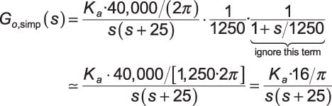
The last line is the reduced-order model for the open-loop system function.