
If you can use a second-order differential equation to describe the circuit you’re looking at, then you’re dealing with a second-order circuit. Circuits that include an inductor, capacitor, and resistor connected in series or in parallel are second-order circuits. Here are second-order circuits driven by an input source, or forcing function.
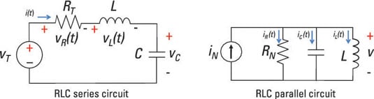
Getting a unique solution to a second-order differential equation requires knowing the initial states of the circuit. For a second-order circuit, you need to know the initial capacitor voltage and the initial inductor current. Knowing these states at time t = 0 provides you with a unique solution for all time after time t = 0.
Use these steps when solving a second-order differential equation for a second-order circuit:
Find the zero-input response by setting the input source to 0, such that the output is due only to initial conditions.
Find the zero-state response by setting the initial conditions equal to 0, such that the output is due only to the input signal.
Zero initial conditions means you have 0 initial capacitor voltage and 0 initial inductor current.
The zero-state response requires you to find the homogeneous and particular solutions:
Homogeneous solution: When there’s no input signal or forcing function — that is, when vT(t) = 0 or iN(t) = 0 — you have the homogeneous solution.
Particular solution: When you have a nonzero input, the solution follows the form of the input signal, giving you the particular solution. For example, if your input is a constant, then your particular solution is also a constant. Likewise, if you have a sine or cosine function as an input, then the output is a combination of sine and cosine functions.
Add up the zero-input and zero-state responses to get the total response.
Because you’re dealing with linear circuits, you want to use superposition to find the total response.
To find the total response for a second-order differential equation with constant coefficients, you should first find the homogeneous solution by using an algebraic characteristic equation and assume the solutions are exponential functions. The roots to the characteristic equation give you the constants found in the exponent of the exponential function.
Guess at an elementary solution: The natural exponential function
This is just one approach to solving second-order circuits. The good news is that it converts a problem involving a differential equation to one that uses only algebra.
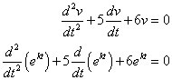
Consider the following differential equation as a numerical example with zero forcing function vT(t) = 0:
The solution to this differential equation is called the homogeneous solution v(t). One classic approach entails giving your best shot at guessing the solution. Try v(t) = ekt. The exponential function works for a first-order equation, so it should work for a second-order equation, too.
When you take the derivative of the natural exponential ekt, you get the same thing multiplied by some constant k. You see how the exponential function is your true amigo in solving differential equations like this.
From calculus to algebra: Using the characteristic equation
To solve a homogeneous differential equation, you can convert the differential equation into a characteristic equation, which you solve using algebra. You do this by substituting your guess v(t) = ekt from earlier into the homogeneous differential equation:
Factoring out ekt leads you to a characteristic equation:
(k2 + 5k +6)ekt = 0
The coefficient of ekt must be 0, so you can solve for k as follows:
k2 + 5k + 6 = 0
k = -2. -3
Setting the algebraic equation to 0 gives you a characteristic equation. The constant roots –2 and –3 determine the features of the solution v(t).
From these roots, you get a homogeneous solution that’s a combination of the solutions e–2t and e–3t:
v(t) = c1e-2t + c2e-3t
The constants c1 and c2 are determined by the initial conditions when t = 0.