The goal of many statistical surveys and studies is to compare two populations, such as men versus women, low versus high-income families, and Republicans versus Democrats. When the characteristic being compared is numerical (for example, height, weight, or income), the object of interest is the amount of difference in the means (averages) for the two populations.
For example, you may want to compare the difference in the average age of Republicans versus Democrats, or the difference in average incomes of men versus women. You estimate the difference between two population means,
by taking a sample from each population (say, sample 1 and sample 2) and using the difference of the two sample means
plus or minus a margin of error. The result is a confidence interval for the difference between two population means,
If both of the population standard deviations are known, then the formula for a CI for the difference between two population means (averages) is
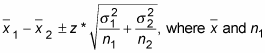
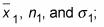
are the mean and size of the first sample, and the first population’s standard deviation,
is given (known);
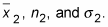
and n2 are the mean and size of the second sample, and the second population’s standard deviation,
is given (known). Here z* is the appropriate value from the standard normal distribution for your desired confidence level. (Refer to the following table for values of z* for certain confidence levels.)
| z*-values for Various Confidence Levels | |
| Confidence Level | z*-value |
|---|---|
| 80% | 1.28 |
| 90% | 1.645 (by convention) |
| 95% | 1.96 |
| 98% | 2.33 |
| 99% | 2.58 |
-
Determine the confidence level and find the appropriate z*-value.
Refer to the above table.
-
Identify
Identify
-
Find the difference,

between the sample means.
-
Square

and divide it by n1; square

and divide it by n2.
Add the results together and take the square root.
-
Multiply your answer from Step 4 by z*.
This answer is the margin of error.
-
Take

plus or minus the margin of error to obtain the CI.
The lower end of the CI is

minus the margin of error, whereas the upper end of the CI is

plus the margin of error.
-
Because you want a 95 percent confidence interval, your z* is 1.96.
-
Suppose your random sample of 100 cobs of the Corn-e-stats variety averages 8.5 inches, and your random sample of 110 cobs of Stats-o-sweet averages 7.5 inches. So the information you have is:

-
The difference between the sample means,

from Step 2, is 8.5 – 7.5 = +1 inch. This means the average for Corn-e-stats minus the average for Stats-o-sweet is positive, making Corn-e-stats the larger of the two varieties, in terms of this sample. Is that difference enough to generalize to the entire population, though? That’s what this confidence interval is going to help you decide.
-
Square

(0.35) to get 0.1225; divide by 100 to get 0.0012. Square

(0.45); divide by 110 to get 0.0018. The sum is 0.0012 + 0.0018 = 0.0030; the square root is 0.0554 inches (if no rounding is done).
-
Multiply 1.96 times 0.0554 to get 0.1085 inches, the margin of error.
-
Your 95 percent confidence interval for the difference between the average lengths for these two varieties of sweet corn is 1 inch, plus or minus 0.1085 inches. (The lower end of the interval is 1 – 0.1085 = 0.8915 inches; the upper end is 1 + 0.1085 = 1.1085 inches.) Notice all the values in this interval are positive. That means Corn-e-stats is estimated to be longer than Stats-o-sweet, based on your data.
To interpret these results in the context of the problem, you can say with 95 percent confidence that the Corn-e-stats variety is longer, on average, than the Stats-o-sweet variety, by somewhere between 0.8915 and 1.1085 inches, based on your sample.
Notice that you could get a negative value for
For example, if you had switched the two varieties of corn, you would have gotten –1 for this difference. You would say that Stats-o-sweet averaged one inch shorter than Corn-e-stats in the sample (the same conclusion stated differently).
If you want to avoid negative values for the difference in sample means, always make the group with the larger sample mean your first group — all your differences will be positive.
However, even if the group with the larger sample mean serves as the first group, sometimes you will still get negative values in the confidence interval. Suppose in the above example that the sample mean of Corn-e-stats was 7.6 inches. Thus, the difference in sample means is 0.1, and the upper end of the confidence interval is 0.1 + 0.1085 = 0.2085 while the lower end is 0.1 – 0.1085 = –0.0085. This means that the true difference is reasonably anywhere from Corn-e-stats being as much as 0.2085 inches longer to Stat-o-sweet being 0.0085 inches longer. It’s too close to tell for sure which variety is longer on average.