After the system has been linearized, a system block diagram utilizing Laplace transform (LT) techniques for feedback control of the vehicle velocity can be constructed. The differential equation can now be taken to the s-domain by taking the Laplace transform (LT) of both sides.
Taking the LT of all time domain quantities produces corresponding s-domain quantities. Of special note the LT of the derivative term, under zero initial conditions, results in s times the transformed quantity and the LT of a step function is 1/s:
Finally you can solve for
in terms of the throttle input
and hill onset gθ:
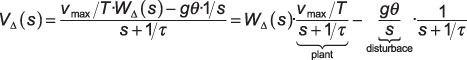
The final equation rewrite on the right, identifies what is known as the plant, in this case the linearized system function for the vehicle dynamics, along with the disturbance gθ term due to hill onset at t = 0. Note the disturbance enters the plant without the inclusion of the gain term vmax/T.
The system block diagram, including a controller to drive the throttle setting and a sensor to feedback the vehicle velocity, is shown in the figure.
![[Credit: Illustration by Mark Wickert, PhD]](https://www.dummies.com/wp-content/uploads/379658.image4.jpg)
The subscript delta has been dropped on the signals W(s) and V(s) with the understanding that these quantities represent throttle and velocity deviations away from the nominal throttle and velocity settings, respectively. For the controller, a proportional-integral (PI) building block is used, with gain constants Kp for the proportional path and Ki for the integral path. This controller is quite common in control systems.
Note in a PI controller the proportional and integral functions are in parallel.
The block diagram input is R(s), which is the LT of r(t), the command input to the cruise control. The command input represents the user input, that is setting the desired vehicle velocity to v0 mph.
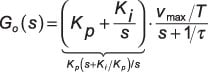
What remains is to find the closed-loop system function H(s) = V(s) / R(s). You start from the open-loop system function, G0(s), which is the product of the s-domain system functions in cascade from input to output, with the feedback removed and the disturbance set to zero:
With the velocity sensor feedback connected, the output V(s) is just [R(s) – V(s)] at the summer output (far left) times G0(s). Solving for the ratio V(s)/R(s) gives you the closed-loop response:
where on the right G0(s) is inserted and the following substitutions made:
The standard form for a second-order denominator is
where ωn is the natural frequency in rad/s and z is the damping factor. Equating terms between the two denominators results in the design equations
To study the impact of hill onset on the cruise control, you need the system function relating the error signal E(s) to the disturbance input Θ(s) when R(s) = 0. Working from V(s) initially,
Because E(s) = –V(s) when R(s) = 0 (zero because the command deviation is zero by assumption), the preceding result holds for E(s) with a sign change. The custom Python function cruise_control(wn,zeta,T, vcruise,vmax,tf_mode) calculates system function b and a coefficient arrays for H(s), E(s) / Θ(s), E(s) / R(s), and W(s) / R(s). Access the function in the module ssd.py.