
The system block diagram for the sled (coarse laser position) control system on a CD/DVD drive is composed of several subsystems. Start with a continuous-time linear time-invariant (LTI) system model of the drive motor and mechanical attributes of the sled drive train (which includes screw gear and sled track). The motor is a heterogeneous system with an electrical signal input; the output is the motor shaft radial position.
The system is dynamical, meaning that the input circuit has a differential equation relationship between the input signal and the shaft rotation. The mechanical side is also dynamical, because of a moment of inertia associated with the load coupled to the motor shaft and the friction associated with the shaft bearings, the screw gear assembly, and sled track.
To figure out how to manage these details in a real-world situation, you’d likely work with a mechanical engineer.
The figure shows the complete LTI system model along with its s-domain system function, which relates the output θ(t) to the input va(t) in the s-domain.
![[Credit: Illustration by Mark Wickert, PhD]](https://www.dummies.com/wp-content/uploads/379079.image0.jpg)
Motor circuit: The upper-left portion is a circuit model of the sled motor. To rotate the motor, you apply a control input signal, the voltage va(t) or, if you’re working in the s-domain, the Laplace transform (LT) of the voltage signal
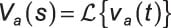
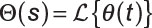
Motor shaft: The voltage across the motor armature winding resistance Ra and series inductance La produces a current that results in electromotive force, which causes the shaft to rotate. The shaft rotation is modeled by the angle θ(t) or, in the s-domain,
A mechanical model of the sled motor includes the equivalent load moment of inertia J and the friction b.
The preceding figure shows a small armature-controlled DC motor, representative of small motors found in computer electronics. The system function for the motor contains the dynamics (differential equation impacts) of both the electrical and mechanical aspects of the motor.
The 1/s term in the model shown — 1/s corresponds to integration in the time domain — converts rotational velocity to rotational position. Without the 1/s in the motor, the output is rotational velocity, which would be useful in modeling a speed control system but not in a CD/DVD player.
The motor system function contains five constants to model the electrical and mechanical attributes of this system:
J = equivalent inertia of the screw drive and sled (
) b = equivalent friction of the screw drive and sled (kg/m/s)
L = armature inductance (mH)
R = armature resistance (Ohms)
Km = motor constant (N x m/A)
With numbers placed into the model for the five motor constants, the motor system function, denoted as
becomes
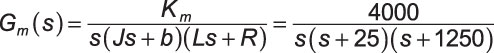
The electrical side is responsible for a pole at s = –1,250 rad/s. The mechanical side has a pole at s = –25 rad/s. Poles represent the denominator polynomial of Gm(s) = 0.
In this model, assume that the tracking sensor operates independently of any other control system for the disc. Check out the complete sled position system block diagram.
![[Credit: Illustration by Mark Wickert, PhD]](https://www.dummies.com/wp-content/uploads/379084.image5.jpg)
The input signal r(t) — R(s) in the s-domain — commands the sled to a new position. The output y(t) — Y(s) w in the s-domain — represents the linear position of the sled.
Think of the system model as two separate parts: the portion you design (controller) and the portion you’re given to work with (plant). The plant, by the way, also includes the screw gear that converts angular position into linear position with the constant of 10/(2π) mm/rad.
A track sensor has a system function of Gts(s) = 1 and measures the linear position of the sled to produce what’s known as a feedback signal. Subtract the feedback signal from the desired position input to form the error signal e(t) — E(s). The error signal is amplified by gain Ka and fed to the controller.
With the track sensor disconnected, r(t) directly controls y(t) through a cascade of system blocks, namely the controller followed by the plant. By extending the LT convolution theorem to multiple system functions, the output Y(s) can be written in terms of the input R(s):
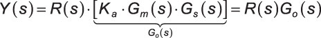
In the language of control systems, G0(s) is known as the open-loop system function. The free variable in this design is the amplifier gain Ka.
With the track sensor switch connected (feedback loop closed), you can now characterize the closed-loop system performance by solving for the system function between R(s) and Y(s) with feedback present. To do that, write an algebraic expression in the s-domain that takes advantage of the linear time-invariant (LTI) nature of all the blocks in the system.
Working from the left side of the block diagram to the right, use the s-domain version of the convolution theorem to write an equation for Y(s) that allows you to solve for the system closed-loop function H(s) = Y(s)/R(s). A series of five steps gets you there:
Write an s-domain expression for the error signal E(s). The preceding figure shows inputs to the summing block on the far left R(s) and –Y(s), so E(s) = R(s) –Y(s).
Write an s-domain expression for the input to the motor by accounting for the amplifier gain Ka: Va(s) = Ka [R(s) –Y(s)].
Develop an s-domain expression for motor rotational position È(s). The convolution theorem reveals that È(s) = Va(s) x Gm(s). Making substitutions generates this equation:

Express the output of the screw gear, which is the desired linear position output:

Solve for the closed-loop system function H(s) = Y(s)/R(s), using the result of Step 4 with the open-loop system function substituted to keep the math cleaner:
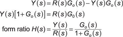
This is a well-known result for feedback systems employing unity gain, Gts(s) = 1, in the feedback path. It shows that the closed-loop system function is the open-loop system function divided by one plus the open-loop system function.