


Regression analysis is one of the most important statistical techniques for business applications. It's a statistical methodology that helps estimate the strength and direction of the relationship between two or more variables. The analyst may use regression analysis to determine the actual relationship between these variables by looking at a corporation's sales and profits over the past several years. The regression results show whether this relationship is valid.
In addition to sales, other factors may also determine the corporation's profits, or it may turn out that sales don't explain profits at all. In particular, researchers, analysts, portfolio managers, and traders can use regression analysis to estimate historical relationships among different financial assets. They can then use this information to develop trading strategies and measure the risk contained in a portfolio.
Regression analysis is an indispensable tool for analyzing relationships between financial variables. For example, it can:
Identify the factors that are most responsible for a corporation's profits
Determine how much a change in interest rates will impact a portfolio of bonds
Develop a forecast of the future value of the Dow Jones Industrial Average
The following ten sections describe the steps used to implement a regression model and analyze the results.
Step 1: Specify the dependent and independent variable(s)
To implement a regression model, it's important to correctly specify the relationship between the variables being used. The value of a dependent variable is assumed to be related to the value of one or more independent variables. For example, suppose that a researcher is investigating the factors that determine the rate of inflation. If the researcher believes that the rate of inflation depends on the growth rate of the money supply, he may estimate a regression model using the rate of inflation as the dependent variable and the growth rate of the money supply as the independent variable.
A regression model based on a single independent variable is known as a simple regression model; with two or more independent variables, the model is known as a multiple regression model.
Step 2: Check for linearity
One of the fundamental assumptions of regression analysis is that the relationship between the dependent and independent variables is linear (i.e., the relationship can be illustrated with a straight line.) One of the quickest ways to verify this is to graph the variables using a scatter plot. A scatter plot shows the relationship between two variables with the dependent variable (Y) on the vertical axis and the independent variable (X) on the horizontal axis.
For example, suppose that an analyst believes that the excess returns to Coca-Cola stock depend on the excess returns to the Standard and Poor's (S&P) 500. (The excess return to a stock equals the actual return minus the yield on a Treasury bill.) Using monthly data from September 2008 through August 2013, the following image shows the excess returns to the S&P 500 on the horizontal axis, whereas the excess returns to Coca-Cola are on the vertical axis.
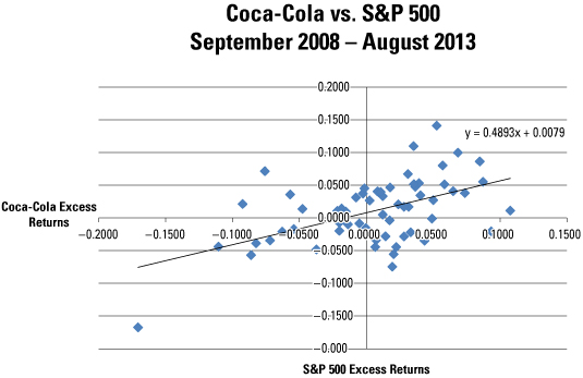
It can be seen from the scatter plot that this relationship is at least approximately linear. Therefore, linear regression may be used to estimate the relationship between these two variables.
Step 3: Check alternative approaches if variables are not linear
If the specified dependent (Y) and independent (X) variables don't have a linear relationship between them, it may be possible to transform these variables so that they do have a linear relationship. For example, it may be that the relationship between the natural logarithm of Y and X is linear. Another possibility is that the relationship between the natural logarithm of Y and the natural logarithm of X is linear. It's also possible that the relationship between the square root of Y and X is linear.
If these transformations don't produce a linear relationship, alternative independent variables may be chosen that better explain the value of the dependent variable.
Step 4: Estimate the model
The standard linear regression model may be estimated with a technique known as ordinary least squares. This results in formulas for the slope and intercept of the regression equation that "fit" the relationship between the independent variable (X) and dependent variable (Y) as closely as possible.
For example, the following tables show the results of estimating a regression model for the excess returns to Coca-Cola stock and the S&P 500 over the period September 2008 through August 2013.
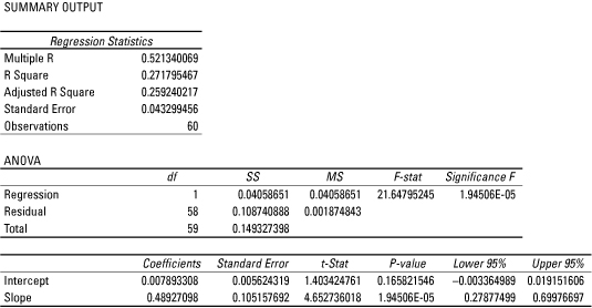
In this model, the excess returns to Coca-Cola stock are the dependent variable, while the excess returns to the S&P 500 are the independent variable. Under the Coefficients column, it can be seen that the estimated intercept of the regression equation is 0.007893308, and the estimated slope is 0.48927098.
Steps 5: Test the fit of the model using the coefficient of variation
The coefficient of variation (also known as R2) is used to determine how closely a regression model "fits" or explains the relationship between the independent variable (X) and the dependent variable (Y). R2 can assume a value between 0 and 1; the closer R2 is to 1, the better the regression model explains the observed data.
As shown in the tables from Step 4, the coefficient of variation is shown as "R-Square"; this equals 0.271795467. The fit isn't particularly strong. Most likely, the model is incomplete, such as factors other than the excess returns to the S&P 500 also determine or explain the excess returns to Coca-Cola stock.
For a multiple regression model, the adjusted coefficient of determination is used instead of the coefficient of determination to test the fit of the regression model.
Step 6: Perform a joint hypothesis test on the coefficients
A multiple regression equation is used to estimate the relationship between a dependent variable (Y) and two or more independent variables (X). When implementing a multiple regression model, the overall quality of the results may be checked with a hypothesis test. In this case, the null hypothesis is that all the slope coefficients of the model equal zero, with the alternative hypothesis that at least one of the slope coefficients is not equal to zero.
If this hypothesis can't be rejected, the independent variables do not explain the value of the dependent variable. If the hypothesis is rejected, at least one of the independent variables does explain the value of the dependent variable.
Step 7: Perform hypothesis tests on the individual regression coefficients
Each estimated coefficient in a regression equation must be tested to determine if it is statistically significant. If a coefficient is statistically significant, the corresponding variable helps explain the value of the dependent variable (Y). The null hypothesis that's being tested is that the coefficient equals zero; if this hypothesis can't be rejected, the corresponding variable is not statistically significant.
This type of hypothesis test can be conducted with a p-value (also known as a probability value.) The tables in Step 4 show that the p-value associated with the slope coefficient is 1.94506 E-05. This expression is written in terms of scientific notation; it can also be written as 1.94506 X 10⁻⁵ or 0.0000194506.
The p-value is compared to the level of significance of the hypothesis test. If the p-value is less than the level of significance, the null hypothesis that the coefficient equals zero is rejected; the variable is, therefore, statistically significant.
In this example, the level of significance is 0.05. The p-value of 0.0000194506 indicates that the slope of this equation is statistically significant; for example, the excess returns to the S&P 500 explain the excess returns to Coca-Cola stock.
Step 8: Check for violations of the assumptions of regression analysis
Regression analysis is based on several key assumptions. Violations of these assumptions can lead to inaccurate results. Three of the most important violations that may be encountered are known as: autocorrelation, heteroscedasticity and multicollinearity.
Autocorrelation results when the residuals of a regression model are not independent of each other. (A residual equals the difference between the value of Y predicted by a regression equation and the actual value of Y.)
Autocorrelation can be detected from graphs of the residuals or by using more formal statistical measures such as the Durbin-Watson statistic. Autocorrelation may be eliminated with appropriate transformations of the regression variables.
Heteroscedasticity refers to a situation where the variances of the residuals of a regression model are not equal. This problem can be identified with a plot of the residuals; transformations of the data may sometimes be used to overcome this problem.
Multicollinearity is a problem that can arise only with multiple regression analysis. It refers to a situation where two or more of the independent variables are highly correlated with each other. This problem can be detected with formal statistical measures, such as the variance inflation factor (VIF). When multicollinearity is present, one of the highly correlated variables must be removed from the regression equation.
Step 9: Interpret the results
The estimated intercept and coefficient of a regression model may be interpreted as follows. The intercept shows what the value of Y would be if X were equal to zero. The slope shows the impact on Y of a change in X.
Based on the tables in Step 4, the estimated intercept is 0.007893308. This indicates that the excess monthly return to Coca-Cola stock would be 0.007893308 or 0.7893308 percent, if the excess monthly return to the S&P 500 were 0 percent.
Also, the estimated slope is 0.48927098. This indicates that a 1 percent increase in the excess monthly return to the S&P 500 would result in a 0.48927098 percent increase in the excess monthly return to Coca-Cola stock. Equivalently, a 1 percent decrease the excess monthly return to the S&P 500 would result in a 0.48927098 percent decrease in the excess monthly return to Coca-Cola stock.
Step 10: Forecast future values
An estimated regression model may be used to produce forecasts of the future value of the dependent variable. In this example, the estimated equation is:
Suppose that an analyst has reason to believe that the excess monthly return to the S&P 500 in September 2013 will be 0.005 or 0.5 percent. The regression equation can be used to predict the excess monthly return to Coca-Cola stock as follows:
The predicted excess monthly return to Coca-Cola stock is 0.010339663 or 1.0339663 percent.

