
Using the ordinary least squares (OLS) technique to estimate a model with a dummy dependent variable is known as creating a linear probability model, or LPM. LPMs aren’t perfect. Three specific problems can arise:
Non-normality of the error term
Heteroskedastic errors
Potentially nonsensical predictions
Non-normality of the error term
The assumption that the error is normally distributed is critical for performing hypothesis tests after estimating your econometric model.
The error term of an LPM has a binomial distribution instead of a normal distribution. It implies that the traditional t-tests for individual significance and F-tests for overall significance are invalid.
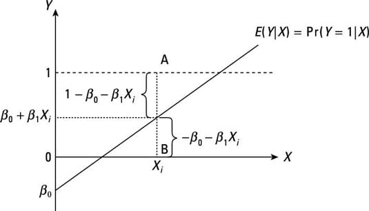
As you can see, the error term in an LPM has one of two possible values for a given X value. One possible value for the error (if Y = 1) is given by A, and the other possible value for the error (if Y = 0) is given by B. Consequently, it’s impossible for the error term to have a normal distribution.
Heteroskedasticity
The classical linear regression model (CLRM) assumes that the error term is homoskedastic. The assumption of homoskedasticity is required to prove that the OLS estimators are efficient (or best). The proof that OLS estimators are efficient is an important component of the Gauss-Markov theorem. The presence of heteroskedasticity can cause the Gauss-Markov theorem to be violated and lead to other undesirable characteristics for the OLS estimators.
The error term in an LPM is heteroskedastic because the variance isn’t constant. Instead, the variance of an LPM error term depends on the value of the independent variable(s).
Using the structure of the LPM, you can characterize the variance of its error term as follows
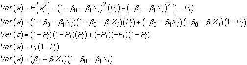
Because the variance of the error depends on the value of X, it exhibits heteroskedasticity rather than homoskedasticity.
Unbounded predicted probabilities
The most basic probability law states that the probability of an event occurring must be contained within the interval [0,1]. But the nature of an LPM is such that it doesn’t ensure this fundamental law of probability is satisfied. Although most of the predicted probabilities from an LPM have sensible values (between 0 and 1), some predicted probabilities may have nonsensical values that are less than 0 or greater than 1.
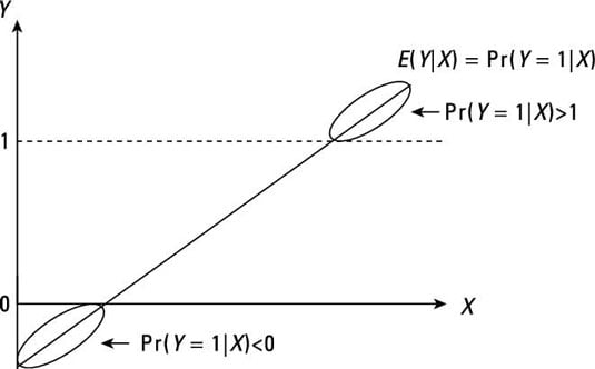
Take a look at the following figure and focus your attention on the segments of the regression line where the conditional probability is greater than 1 or less than 0. When the dependent variable is continuous, you don’t have to worry about unbounded values for the conditional means. However, dichotomous variables are problematic because the conditional means represent conditional probabilities. Interpreting probabilities that aren’t bounded by 0 and 1 is difficult.
You can see an example of this problem with actual data:
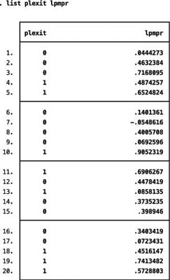
Most of the estimated probabilities from the LPM estimation are contained within the [0,1] interval, but the predicted probability for the seventh observation is negative. Unfortunately, nothing in the estimation of an LPM ensures that all the predicted probabilities stay within reasonable values.