Working across Domains Example: Take the RC Low-Pass Filter to the Z-Domain

Working across domains is a fact of life as a computer and electronic engineer. Solving real computer and electrical engineering tasks requires you to assimilate the vast array of signals and systems concepts and techniques and apply them in a smart and efficient way. Here’s an example problem that shows how analysis and modeling across the time, frequency, and s- and z-domains actually works.

This example works across continuous- and discrete-time systems.

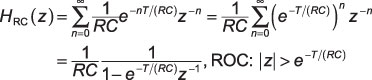
The series resistor shunt capacitor (RC) low-pass filter is an example of an LTI system that’s represented by a first-order LCC differential equation. Here’s the formula for the impulse response and system function:

RC is the time constant associated with the series resistor and shunt capacitor that defines the filter circuit. This problem asks you to find a simple discrete-time filter equivalent.

Suppose h[n] = h(nT) = h(n/f_s). The Laplace transform (LT) of h(t) following sampling is

This result indicates that sampling a continuous-time impulse response maps the s-plane to the z-plane via z = e^sT. (This connection is part of the figure.) For the RC filter impulse response in particular, the pole at s = –1/(RC) is mapped to a pole at z = e^–T/RC in the z-plane.

Because e^–T/(RC) < 1, the pole is stable. Formally, this is called an impulse invariant filter design, and it allows you to transfer a continuous-time filter to the discrete-time domain.

In the broader sense, the z = e^sT transformation maps the left-half s-plane to the interior of the unit circle in the z-plane and the right-half s-plane to the exterior of the unit circle in the z-plane. The jω-axis of the s-plane maps to the unit circle, which is where jω resides in the z-plane.

The mapping occurs repeatedly because of sampling theory. Aliasing of the filter frequency response also occurs, unless it’s bandlimited (zero) for f > f_s/2.

To complete the filter design, place the sampled impulse response in the z-transform definition:

Fine-tune the design for implementation

This filter is like h[n] = aⁿu[n] for 0 < a < 1, with the scale factor 1/(RC) and a = e^–T/(RC). One detail remains that the design procedure hasn’t taken care of, and that’s ensuring that the filter gain at frequencies is preserved, in particular f = 0.

In the continuous-time domain, this means finding H(s = j0) = 1/(RC)/[j0 + 1/(RC)] = 1 and choosing a gain factor G to place in front of H_RC(z) to force the gain to also be one at z = e^j0 = 1:

In the end, with G value included, you have

To actually implement this filter in an application, you need the difference equation representation of this filter. The system function is the ratio of output over the input in the z-domain: H_RC(z) = Y(z)/X(z). To find the difference equation, you first need to cross-multiply X(z) times the numerator of H_RC(z) on the right and cross-multiply the denominator times X(z) on the left:

Next, apply the inverse z-transform on the left and right sides, using the linearity and delay properties of the z-transform:

Make the Python frequency response comparison

Use Python to take a quick look at the frequency response magnitude of the original analog filter and the digital filter realization. The analog low-pass filter time constant is related to the filter 3dB cutoff frequency (where 20log₁₀|H(f_3dB)| = –3.0) via f_3dB = 1/(2πRC).

Here, set f_3dB = 100 Hz and sweep the frequency logarithmically from 0.1 Hz to 100 kHz. Set the sampling rate f_s = 1/T = 200 KHz and recognize that the digital filter will be useful only for 0 ≤ f ≤ f_s/2 in hertz or the following in radians per sample:

The frequency response magnitude in dB for both filters is shown in the following figure. Note in particular the responses overlap except when f is very close to the 100-kHz folding frequency.

In [<b>25</b>]: f = logspace(-1,5,500)
In [<b>26</b>]: RC = 1/(2*pi*100)
In [<b>27</b>]: w,Hs = signal.freqs([1/RC],[1,1/RC],2*pi*f)
In [<b>28</b>]: a = exp(-1/(RC*2e5))
In [<b>29</b>]: w,Hz = signal.freqz([1-a],[1, -a],2*pi*f/2e5)
In [<b>30</b>]: semilogx(f,20*log10(abs(Hs)))
In [<b>31</b>]: semilogx(f,20*log10(abs(Hz)))
In [<b>32</b>]: axis([1e-1,1e5,-60,5])

Credit: Illustration by Mark Wickert, PhD

The response comparison between the two filters is good. The fact that the digital filter response lies above the analog response near f_s/2 is due to aliasing in the frequency response. Alternative digital filter design approaches can mitigate this, but not without some tradeoffs. That’s engineering.