In statistics, a sampling distribution is based on sample averages rather than individual outcomes. This makes it different from a distribution. Here’s why: A random variable is a characteristic of interest that takes on certain values in a random manner. For example, the number of red lights you hit on the way to work or school is a random variable; the number of children a randomly selected family has is a random variable. You use capital letters such as X or Y to denote random variables and you use lowercase letters such as x or y to denote actual, observed outcomes of random variables.
A distribution is a listing, graph, or function of all possible outcomes of a random variable (such as X) and how often each actual outcome (x), or set of outcomes, occurs.
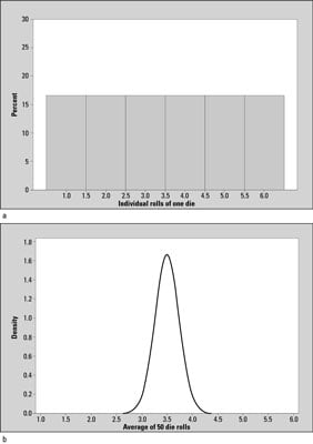
For example, suppose a million of your closest friends each roll a single die and record each actual outcome (x). A table or graph of all these possible outcomes (one through six) and how often they occurred represents the distribution of the random variable X. A graph of the distribution of X in this case is shown in example a in the above figure for Example (a). It shows the numbers 1–6 appearing with equal frequency (each one occurring 1/6 of the time), which is what you expect over many rolls if the die is fair.
Now suppose each of your friends rolls this single die 50 times (n = 50) and records the average value of those 50 rolls,
The graph of all their averages of all their samples represents the distribution of the random variable
Because this distribution is based on sample averages (of size 50) rather than individual outcomes (of size 1), this distribution has a special name. It’s called the sampling distribution of the sample mean,
Example (b) in the above figure shows the sampling distribution of
the average of 50 rolls of a die.
Example (b) (average of 50 rolls) shows the same range (1 through 6) of outcomes as Example (a) (individual rolls), but Example (b) has more possible outcomes. You could get an average of 3.3 or 2.8 or 3.9 for 50 rolls, for example, whereas someone rolling a single die can only get whole numbers from 1 to 6.
Also, the shape of the graphs are different; example a shows a flat, uniform shape, where each outcome is equally likely, and Example (b) has a mound shape; that is, outcomes near the center (3.5) occur with high frequency and outcomes near the edges (1 and 6) occur with extremely low frequency. This is to be expected. If you were to roll a die 50 times, you would expect the average to be near the average of the values 1,2,3,4,5,6 since each of those values are equally likely to occur. The average of 1,2,3,4,5,6 is 3.5.