A probability density function (PDF) shows the probabilities of a random variable for all its possible values. The probabilities associated with specific values (or events) from a random variable must adhere to the properties
where Xj represents the possible values (outcomes) of random variable X. In other words, the chances of any random event occurring must be anywhere from impossible (probability of 0) to certain (probability of 1), and the sum of the probabilities for all events must be 1 (or 100 percent).
The PDF for discrete random variables
If you’re observing a discrete random variable, the PDF can be described in a table or graph. To construct a table, you set up one column with the possible values of your random variable and one column with the probability that they’ll occur.
In a graphical depiction of the PDF (a bar graph), you’d place the possible values of the random variable on the horizontal axis, and the height of the vertical bars at each value show the probability that they occur.
Suppose you perform an experiment that consists of tossing three coins at the same time. You're interested in the number of times they land heads up, so call the number of heads observed random variable X. The table lists the possible outcomes for this experiment and the values for X generated from the process.
| Outcome | First Coin | Second Coin | Third Coin | Number of Heads, X |
|---|---|---|---|---|
| 1 | T | T | T | 0 |
| 2 | T | T | H | 1 |
| 3 | T | H | T | 1 |
| 4 | H | T | T | 1 |
| 5 | T | H | H | 2 |
| 6 | H | H | T | 2 |
| 7 | H | T | H | 2 |
| 8 | H | H | H | 3 |
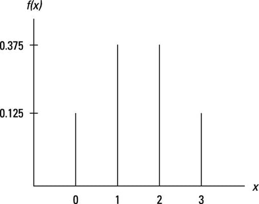
Out of eight possible outcomes, you get 0 heads in one outcome, 1 head in three outcomes, 2 heads in three outcomes, and 3 heads in one outcome. You can summarize the information with a tabular or graphical depiction of the PDF for X.
You see 8 total outcomes and four possible values for X: 0, 1, 2, and 3. This information allows you to calculate the probability associated with each X value. For example, X = 0 occurs only once, so f(X = 0) = 1/8 = 0.125. The following table shows the probabilities for the other X values and a tabular form of the PDF.
| X | f(X) |
|---|---|
| 0 | 1/8 = 0.125 |
| 1 | 3/8 = 0.375 |
| 2 | 3/8 = 0.375 |
| 3 | 1/8 = 0.125 |
Note that the probabilities in the right-hand column add up to 1. The total probabilities for any experiment must always equal 1.
The PDF for continuous random variables
If you’re observing a continuous random variable, the PDF can be described in a function or graph. The function shows how the random variable behaves over any possible range of values. In a graphical depiction of the PDF, the possible values of the random variable are on the horizontal axis, and a curve (without any bars or breaks) is somewhere above the axis.
The most common continuous PDF is that of a normally distributed random variable. The graphical depiction of this PDF is shown here.
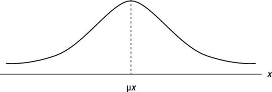
Regardless of the values of the mean and standard deviation, the total density (area) under the curve is equal to 1. In addition, about 68 percent of the density is within one standard deviation, about 95 percent of the density is within two standard deviations, and about 99.7 percent of the density is within three standard deviations.
Because a continuous random variable can take on infinitely many values, the probability that a specific value occurs is zero!
An example can help illustrate this point. Suppose a teacher randomly chooses one of his econometrics students. What is the probability that the student will be exactly 21 years of age? Answer: essentially zero.
The reason is that student would have to be randomly selected at the precise day, hour, minute, second, and fraction of a second that he or she was born 21 years ago. That would be virtually impossible. There would, however, be some chance of randomly selecting a student who’s between the ages of 20 and 22.
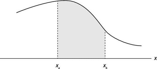
Probabilities with continuous random variables are measured over intervals. Mathematically, this probability measurement is expressed as
where Xa and Xb are possible values that can be taken by the random variable X.