Like putting two people back-to-back to see who’s taller, Sigma Six uses box and whisker plots (or just box plots) to directly compare two or more variation distributions. When you need to compare value distributions for multiple characteristics, few things are quicker to make or easier to interpret than a box and whisker plot.
A box and whisker plot is made up of a box, which represents the central mass of the variation, and thin lines, called whiskers, that extend out on either side and represent the thinning tails of the distribution.
To create a box and whisker plot, just follow these steps:
Rank the data measurements in order from least to greatest.
Determine the median of the data.
Find the observed value in the rank-ordered data where half of the data lies above and half lies below.
When the number of observed points (n) in your data set is odd, take
That value in the rank-ordered sequence is your median. For example, if n equals 99, take 99 + 1 = 100 and then divide that result by 2 to get 50. The 50th number in your list is the median.
When n is even, the median is the average of the

and the
values in the rank-ordered sequence. If n = 100, you’d find 100 ÷ 2 and (100 ÷ 2) + 1. Those expressions give you 50 and 51, so you’d find the 50th and 51st values and average them to find the median.
Find the first quartile, Q1.
The first quartile marks the 25-percent point in your rank-ordered sequence; three-quarters of the data are yet to come.
Find the third quartile, Q3.
The third quartile is the 75-percent point in your rank-ordered sequence; one-quarter of the data is left.
Find the largest observed value, xMAX, and the smallest observed value, xMIN.
Draw a horizontal line, representing the scale of measure for the characteristic.
This scale can be in millimeters for length, pounds for weight, minutes for time, number of defects found on an inspected part, or anything else that quantifies what aspect of the characteristic you’re interested in.
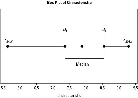
Mark your median and quartile values from Steps 2 through 4 and construct the box.
Make points for your median and quartile values. Draw a box spanning from the first quartile (Q1) to the third quartile (Q3) and draw a vertical line in the box corresponding to the median value.
Add the minimum and maximum values from Step 5 and construct the whiskers.
Draw two horizontal lines, one extending out from the Q1 value to the smallest observed observation, xMIN, and another extending out from the Q3 value to the greatest observed value, xMAX.
Repeat Steps 1 through 8 for each additional characteristic to be plotted and compared against the same horizontal scale.
When you have a large set of data for a characteristic, you may want to extend the whiskers out to only the 10th and 90th percentiles, or to the 5th and 95th percentiles and so on, rather than to the maximum and minimum values. Then when outlier data points fall beyond these ends of the whiskers, you can draw them as disconnected dots or stars.
This method is a great way of graphically identifying and communicating the presence of outliers in your data.
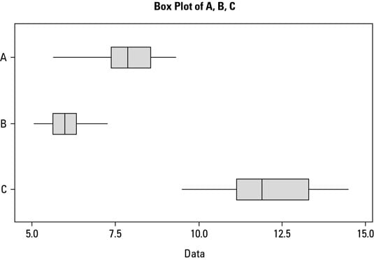
Box and whisker plots are ideal for comparing two or more variation distributions, such as before-and-after views of a process or characteristic or alternative ways of conducting an operation. Essentially, when you want to quickly find out whether two or more variation distributions are different (or the same), you create a box plot.
Distribution B clearly has the lowest level. But it still overlaps the performance of distribution A, indicating that it may not be that different. Distribution C, on the other hand, has a much higher value and no overlap with distributions A and B. It also has a much broader spread to its variation.
Other things to look for in comparative box plots include the following:
Differences or similarities in location of the median
Differences or similarities in box widths
Differences or similarities in whisker-to-whisker spread
Overlap or gaps between distributions
Skewed or asymmetrical variation in distributions
The presence of outliers